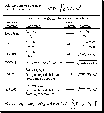
Figure 12. Summary of distance function definitions.
This section compares the distance functions discussed in this paper. A nearest neighbor classifier was implemented using each of six different distance functions: Euclidean (normalized by standard deviation) and HOEM as discussed in Section 2; HVDM as discussed in Section 3; DVDM and IVDM as discussed in Section 4; and WVDM as discussed in Section 5. Figure 12 summarizes the definition of each distance function.
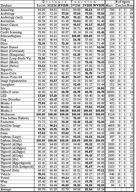
Each distance function was tested on 48 datasets from the UCI machine learning databases, again using 10-fold cross-validation. The average accuracy over all 10 trials is reported for each test in Table 8. The highest accuracy achieved for each dataset is shown in bold. The names of the three new distance functions presented in this paper (HVDM, IVDM and WVDM) are also shown in bold to identify them.
Table 8 also lists the number of instances in each database ("#Inst."), and the number of continuous ("Con"), integer ("Int", i.e., linear discrete), and nominal ("Nom") input attributes.

Figure 12. Summary of distance function definitions.
On this set of 48 datasets, the three new distance functions (HVDM, IVDM and WVDM) did substantially better than Euclidean distance or HOEM. IVDM had the highest average accuracy (85.56%) and was almost 5% higher on average than Euclidean distance (80.78%), indicating that it is a more robust distance function on these datasets, especially those with nominal attributes. WVDM was only slightly lower than IVDM with 85.24% accuracy. Somewhat surprisingly, DVDM was slightly higher than HVDM on these datasets, even though it uses discretization instead of a linear distance on continuous attributes. All four of the VDM-based distance functions outperformed Euclidean distance and HOEM.
Out of the 48 datasets, Euclidean distance had the highest accuracy 11 times; HOEM was highest 7 times; HVDM, 14; DVDM, 19; IVDM, 25 and WVDM, 18.
For datasets with no continuous attributes, all four of the VDM-based distance functions (HVDM, DVDM, IVDM and WVDM) are equivalent. On such datasets, the VDM-based distance functions achieve an average accuracy of 86.6% compared to 78.8% for HOEM and 76.6% for Euclidean, indicating a substantial superiority on such problems.
For datasets with no nominal attributes, Euclidean and HVDM are equivalent, and all the distance functions perform about the same on average except for DVDM, which averages about 4% less than the others, indicating the detrimental effects of discretization. Euclidean and HOEM have similar definitions for applications without any nominal attributes, except that Euclidean is normalized by standard deviation while HOEM is normalized by the range of each attribute. It is interesting that the average accuracy over these datasets is slightly higher for Euclidean than HOEM, indicating that the standard deviation may provide better normalization on these datasets. However, the difference is small (less than 1%), and these datasets do not contain many outliers, so the difference is probably negligible in this case.
 |
Table 8. Summary of Generalization Accuracy
One disadvantage with scaling attributes by the standard deviation is that attributes which almost always have the same value (e.g., a boolean attribute that is almost always 0) will be given a large weight--not due to scale, but because of the relative frequencies of the attribute values. A related problem can occur in HVDM. If there is a very skewed class distribution (i.e., there are many more instances of some classes than others), then the P values will be quite small for some classes and quite large for others, and in either case the difference |Pa,x,c - Pa,y,c| will be correspondingly small, and thus nominal attributes will get very little weight when compared to linear attributes. This phenomenon was noted by Ting (1994, 1996), where he recognized such problems on the hypothyroid dataset. Future research will address these normalization problems and look for automated solutions. Fortunately, DVDM, IVDM and WVDM do not suffer from either problem, because all attributes are scaled by the same amount in such cases, which may in part account for their success over HVDM in the above experiments.
For datasets with both nominal and continuous attributes, HVDM is slightly higher than Euclidean distance on these datasets, which is in turn slightly higher than HOEM, indicating that the overlap metric may not be much of an improvement on heterogeneous databases. DVDM, IVDM and WVDM are all higher than Euclidean distance on such datasets, with IVDM again in the lead.
Distance functions that use VDM require some statistics to determine distance. We therefore hypothesized that generalization accuracy might be lower for VDM-based distance functions than for Euclidean distance or HOEM when there was very little data available, and that VDM-based functions would increase in accuracy more slowly than the others as more instances were made available, until a sufficient number of instances allowed a reasonable sample size to determine good probability values.

Figure 13. Average accuracy as the amount of data increases.
To test this hypothesis, the experiments used to obtain the results shown in Table 8 were repeated using only part of the available training data. Figure 13 shows how the generalization accuracy on the test set improves as the percentage of available training instances used for learning and generalization is increased from 1% to 100%. The generalization accuracy values shown are the averages over all 48 of the datasets in Table 8.
Surprisingly, the VDM-based distance functions increased in accuracy as fast or faster than Euclidean and HOEM even when there was very little data available. It may be that when there is very little data available, the random positioning of the sample data in the input space has a greater detrimental affect on accuracy than does the error in statistical sampling for VDM-based functions.
It is interesting to note from Figure 13 that the six distance functions seem to pair up into three distinct pairs. The interpolated VDM-based distance functions (IVDM and WVDM) maintain the highest accuracy, the other two VDM-based functions are next, and the functions based only on linear and overlap distance remain lowest from very early in the graph.
This section considers the storage requirements, learning speed, and generalization speed of each of the algorithms presented in this paper.
All of the above distance functions must store the entire training set, requiring O(nm) storage, where n is the number of instances in the training set and m is the number of input attributes in the application, unless some instance pruning technique is used. For the Euclidean and HOEM functions, this is all that is necessary, but even this amount of storage can be restrictive as n grows large.
For HVDM, DVDM, and IVDM, the probabilities Pa,x,c for all m attributes (only discrete attributes for HVDM) must be stored, requiring O(mvC) storage, where v is the average number of attribute values for the discrete (or discretized) attributes and C is the number of output classes in the application. It is possible to instead store an array Da,x,y = vdma(x,y) for HVDM and DVDM, but the storage would be O(mv2), which is only a savings when C < v.
For WVDM, C probability values must be stored for each continuous attribute value, resulting in O(nmC) storage which is typically much larger than O(mvC) because n is usually much larger than v (and cannot be less). It is also necessary to store a list of (pointers to) instances for each attribute, requiring an additional O(mn) storage. Thus the total storage for WVDM is O((C+2)nm) = O(Cnm).

Table 9. Summary of efficiency for six distance metrics.
Table 9 summarizes the storage requirements of each system. WVDM is the only one of these distance functions that requires significantly more storage than the others. For most applications, n is the critical factor, and all of these distance functions could be used in conjunction with instance pruning techniques to reduce storage requirements. See Section 7 for a list of several techniques to reduce the number of instances retained in the training set for subsequent generalization.
It takes nm time to read in a training set. It takes an additional 2nm time to find the standard deviation of the attributes for Euclidean distance, or just nm time to find the ranges for HOEM.
Computing VDM statistics for HVDM, DVDM and IVDM takes mn+mvC time, which is approximately O(mn). Computing WVDM statistics takes mnlogn+mnC time, which is approximately O(mnlogn).
In general, the learning time is quite acceptable for all of these distance functions.
Assuming that each distance function must compare a new input vector to all training instances, Euclidean and HOEM take O(mn) time. HVDM, IVDM and DVDM take O(mnC) (unless Da,x,y has been stored instead of Pa,x,c for HVDM, in which case the search is done in O(mn) time). WVDM takes O(logn+mnC) = O(mnC) time.
Though m and C are typically fairly small, the generalization process can require a significant amount of time and/or computational resources as n grows large. Techniques such as k-d trees (Deng & Moore, 1995; Wess, Althoff & Derwand, 1994; Sproull, 1991) and projection (Papadimitriou & Bentley, 1980) can reduce the time required to locate nearest neighbors from the training set, though such algorithms may require modification to handle both continuous and nominal attributes. Pruning techniques used to reduce storage (as in Section 6.2.1) will also reduce the number of instances that must be searched for generalization.
Return to Contents
Send comments to randy@axon.cs.byu.edu