 |
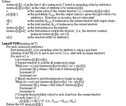
Figure 9. Pseudo code for the WVDM learning algorithm.
The IVDM algorithm can be thought of as sampling the value of
Pa,u,c at the midpoint mida,u of each
discretized range u. P is sampled by first finding the instances
that have a value for attribute a in the range
mida,u +/- wa / 2.
Na,u is incremented once for each such instance, and
Na,u,c is also incremented for each instance whose output
class is c, after which
Pa,u,c = Na,u,c / N
Figure 9 shows pseudo-code for the Windowed Value Difference Metric (WVDM). The WVDM samples the value of Pa,x,c at each value x occurring in the training set for each attribute a, instead of only at the midpoints of each range. In fact, the discretized ranges are not even used by WVDM on continuous attributes, except to determine an appropriate window width, wa, which is the same as the range width used in DVDM and IVDM.
For each value x occurring in the training set for attribute a,
P is sampled by finding the instances that have a value for attribute
a in the range
x +/- wa / 2, and then computing
Na,x, Na,x,c, and
Pa,x,c = Na,x,c / N
 |
For each attribute the values are sorted (using an O(nlogn) sorting algorithm) so as to allow a sliding window to be used and thus collect the needed statistics in O(n) time for each attribute. The sorted order is retained for each attribute so that a binary search can be performed in O(log n) time during generalization.
Values occurring between the sampled points are interpolated just as in IVDM, except that there are now many more points available, so a new value will be interpolated between two closer, more precise values than with IVDM.
The pseudo-code for the interpolation algorithm is given in Figure 10. This algorithm takes a value x for attribute a and returns a vector of C probability values Pa,x,c for c=1..C. It first does a binary search to find the two consecutive instances in the sorted list of instances for attribute a that surround x. The probability for each class is then interpolated between that stored for each of these two surrounding instances. (The exceptions noted in parenthesis handle outlying values by interpolating towards 0 as is done in IVDM.)
 |
Once the probability values for each of an input vector's attribute values are computed, they can be used in the vdm function just as the discrete probability values are.
The WVDM distance function is defined as:
 (25)
(25)and wvdma is defined as:
 (26)
(26)
One drawback to this approach is the increased storage needed to retain C probability values for each attribute value in the training set. Execution time is not significantly increased over IVDM or DVDM. (See Section 6.2 for a discussion on efficiency considerations).

Figure 11. Example of the WVDM probability landscape.
Figure 11 shows the probability values for each of the three classes for the first attribute of the Iris database again, this time using the windowed sampling technique. Comparing Figure 11 with Figure 8 reveals that on this attribute IVDM provides approximately the same overall shape, but misses much of the detail. For example, the peak occurring for output class 2 at approximately sepal length=5.75. In Figure 8 there is a flat line which misses this peak entirely, due mostly to the somewhat arbitrary position of the midpoints at which the probability values are sampled.
Table 7 summarizes the results of testing the WVDM algorithm on the same datasets as DVDM and IVDM. A bold entry again indicates the highest of the two accuracy measurements, and an asterisk (*) indicates a difference that is statistically significant at the 90% confidence level, using a two-tailed paired t-test.

Table 7. Generalization accuracy of WVDM vs. DVDM.
On this set of databases, WVDM was an average of 1.6% more accurate than DVDM overall. WVDM had a higher average accuracy than DVDM on 23 out of the 34 databases, and was significantly higher on 9, while DVDM was only higher on 11 databases, and none of those differences were statistically significant.
Section 6 provides further comparisons of WVDM with other distance functions, including IVDM.
Return to Contents
Send comments to randy@axon.cs.byu.edu