4. Interpolated Value Difference Metric (IVDM)

In this section and Section 5 we introduce distance functions that allow VDM to be applied directly to continuous attributes. This alleviates the need for normalization between attributes. It also in some cases provides a better measure of distance for continuous attributes than linear distance.

For example, consider an application with an input attribute height and an output class that indicates whether a person is a good candidate to be a fighter pilot in a particular airplane. Those individuals with heights significantly below or above the preferred height might both be considered poor candidates, and thus it could be beneficial to consider their heights as more similar to each other than to those of the preferred height, even though they are farther apart in a linear sense.

On the other hand, linear attributes for which linearly distant values tend to indicate different classifications should also be handled appropriately. The Interpolated Value Difference Metric (IVDM) handles both of these situations, and handles heterogeneous applications robustly.

A generic version of the VDM distance function, called the discretized value difference metric (DVDM) will be used for comparisons with extensions of VDM presented in this paper.

4.1. IVDM Learning Algorithm

The original value difference metric (VDM) uses statistics derived from the training set instances to determine a probability P_a,x,c that the output class is c given the input value x for attribute a.

When using IVDM, continuous values are discretized into s equal-width intervals (though the continuous values are also retained for later use), where s is an integer supplied by the user. Unfortunately, there is currently little guidance on what value of s to use. A value that is too large will reduce the statistical strength of the values of P, while a value too small will not allow for discrimination among classes. For the purposes of this paper, we use a heuristic to determine s automatically: let s be 5 or C, whichever is greatest, where C is the number of output classes in the problem domain. Current research is examining more sophisticated techniques for determining good values of s, such as cross-validation, or other statistical methods (e.g., Tapia & Thompson, 1978, p. 67). (Early experimental results indicate that the value of s may not be critical as long as s >= C and s << n, where n is the number of instances in the training set.)

The width w_a of a discretized interval for attribute a is given by:

(17)

where max_a and min_a are the maximum and minimum value, respectively, occurring in the training set for attribute a.

As an example, consider the Iris database from the UCI machine learning databases. The Iris database has four continuous input attributes, the first of which is sepal length. Let T be a training set consisting of 90% of the 150 available training instances, and S be a test set consisting of the remaining 10%.

In one such division of the training set, the values in T for the sepal length attribute ranged from 4.3 to 7.9. There are only three output classes in this database, so we let s=5, resulting in a width of |7.9 - 4.3| / 5 = 0.72. Note that since the discretization is part of the learning process, it would be unfair to use any instances in the test set to help determine how to discretize the values. The discretized value v of a continuous value x for attribute a is an integer from 1 to s, and is given by:

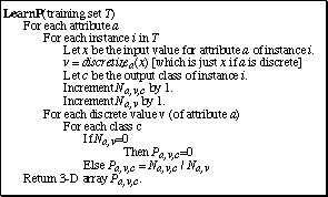
(18)

After deciding upon s and finding w_a, the discretized values of continuous attributes can be used just like discrete values of nominal attributes in finding P_a,x,c. Figure 5 lists pseudo-code for how this is done.

Figure 5. Pseudo code for finding Pa,x,c.

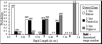
For the first attribute of the Iris database, the values of P_a,x,c are displayed in Figure 6. For each of the five discretized ranges of x, the probability for each of the three corresponding output classes are shown as the bar heights. Note that the heights of the three bars sum to 1.0 for each discretized range. The bold integers indicate the discretized value of each range. For example, a sepal length greater than or equal to 5.74 but less than 6.46 would have a discretized value of 3.

Figure 6. P_a,x,c for a=1, x=1..5, c=1..3, on the first attribute of the Iris database.

4.2. IVDM and DVDM Generalization

Thus far the DVDM and IVDM algorithms learn identically. However, at this point the DVDM algorithm need not retain the original continuous values because it will use only the discretized values during generalization. On the other hand, the IVDM will use the continuous values.

During generalization, an algorithm such as a nearest neighbor classifier can use the distance function DVDM, which is defined as follows:

(19)

where discretize_a is as defined in Equation (18) and vdm_a is defined as in Equation (8), with q=2. [See erratum: Equation (20) should really be a copy of Equation (15), not Equation (8), i.e., it should have a square root over the summation.] We repeat it here for convenience:

(20)

Unknown input values (Quinlan, 1989) are treated as simply another discrete value, as was done in (Domingos, 1995).

Table 4. Example from the Iris database.

As an example, consider two training instances A and B as shown in Table 4, and a new input vector y to be classified. For attribute a=1, the discretized values for A, B, and y are 1, 2, and 2, respectively. Using values from Figure 6, the distance for attribute 1 between y and A is:

while the distance between y and B is 0, since they have the same discretized value.

Note that y and B have values on different ends of range 2, and are not actually nearly as close as y and A are. In spite of this fact, the discretized distance function says that y and B are equal because they happen to fall into the same discretized range.

Figure 7. P_1,x,2 values from the DVDM and IVDM for attribute 1, class 2 of the Iris database.

IVDM uses interpolation to alleviate such problems. IVDM assumes that the P_a,x,c values hold true only at the midpoint of each range, and interpolates between midpoints to find P for other attribute values.

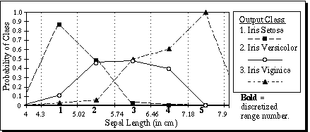
Figure 7 shows the P values for the second output class (Iris Versicolor) as a function of the first attribute value (sepal length). The dashed line indicates what P value is used by DVDM, and the solid line shows what IVDM uses.

The distance function for the Interpolated Value Difference Metric is defined as:

(21)

where ivdm_a is defined as:

(22)

(23)

In this equation, mid_a,u and mid_a,u+1 are midpoints of two consecutive discretized ranges such that mid_a,u <= x < md_a,u+1. P_a,u,c is the probability value of the discretized range u, which is taken to be the probability value of the midpoint of range u (and similarly for P_a,u+1,c). The value of u is found by first setting u = discretize_a(x), and then subtracting 1 from u if x < mid_a,u. The value of mid_a,u can then be found as follows:

(24)

Figure 8 shows the values of p_a,c(x) for attribute a=1 of the Iris database for all three output classes (i.e. c=1, 2, and 3). Since there are no data points outside the range min_a..max_a, the probability value P_a,u,c is taken to be 0 when u < 1 or u > s, which can be seen visually by the diagonal lines sloping toward zero on the outer edges of the graph. Note that the sum of the probabilities for the three output classes sum to 1.0 at every point from the midpoint of range 1 through the midpoint of range 5.

Figure 8. Interpolated probability values for attribute 1 of the Iris database.

Using IVDM on the example instances in Table 4, the values for the first attribute are not discretized as they are with DVDM, but are used to find interpolated probability values. In that example, y has a value of 5.1, so p_1,c(x) interpolates between midpoints 1 and 2, returning the values shown in Table 5 for each of the three classes. Instance A has a value of 5.0, which also falls between midpoints 1 and 2, but instance B has a value of 5.7, which falls between midpoints 2 and 3.

As can be seen from Table 5, IVDM (using the single-attribute distance function ivdm) returns a distance which indicates that y is closer to A than B (for the first attribute), which is certainly the case here. DVDM (using the discretized vdm), on the other hand, returns a distance which indicates that the value of y is equal to that of B, and quite far from A, illustrating the problems involved with using discretization.

Table 5. Example of ivdm vs. vdm.

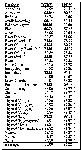
The IVDM and DVDM algorithms were implemented and tested on 48 datasets from the UCI machine learning databases. The results for the 34 datasets that contain at least some continuous attributes are shown in Table 6. (Since IVDM and DVDM are equivalent on domains with only discrete attributes, the results on the remaining datasets are deferred to Section 6.) 10-fold cross-validation was again used, and the average accuracy for each database over all 10 trials is shown in Table 6. Bold values indicate which value was highest for each database. An asterisk (*) indicates that the difference is statistically significant at a 90% confidence level or higher, using a two-tailed paired t-test.

Table 6. Generalization accuracy for DVDM vs. IVDM.

On this set of datasets, IVDM had a higher average generalization accuracy overall than the discretized algorithm. IVDM obtained higher generalization accuracy than DVDM in 23 out of 34 cases, 13 of which were significant at the 90% level or above. DVDM had a higher accuracy in 9 cases, but only one of those had a difference that was statistically significant.

These results indicate that the interpolated distance function is typically more appropriate than the discretized value difference metric for applications with one or more continuous attributes. Section 6 contains further comparisons of IVDM with other distance functions.

Return to Contents