 (11)
(11)
As discussed in the previous section, the Euclidean distance function is inappropriate for nominal attributes, and VDM is inappropriate for continuous attributes, so neither is sufficient on its own for use on a heterogeneous application, i.e., one with both nominal and continuous attributes.
In this section, we define a heterogeneous distance function HVDM that returns the distance between two input vectors x and y. It is defined as follows:
 (11)
(11)
where m is the number of attributes. The function
da(x,y) returns a distance between the two
values x and y for attribute a and is defined
as:
 (12)
(12)The function da(x,y) uses one of two functions (defined below in Section 3.1), depending on whether the attribute is nominal or linear. Note that in practice the square root in (11) is not typically performed because the distance is always positive, and the nearest neighbor(s) will still be nearest whether or not the distance is squared. However, there are some models (e.g., distance-weighted k-nearest neighbor, Dudani, 1976) that require the square root to be evaluated.
Many applications contain unknown input values which must be handled appropriately in a practical system (Quinlan, 1989). The function da(x,y) therefore returns a distance of 1 if either x or y is unknown, as is done by Aha, Kibler & Albert (1991) and Giraud-Carrier & Martinez (1995). Other more complicated methods have been tried (Wilson & Martinez, 1993), but with little effect on accuracy.
The function HVDM is similar to the function HOEM given in Section 2.3, except that it uses VDM instead of an overlap metric for nominal values and it also normalizes differently. It is also similar to the distance function used by RISE 2.0 (Domingos, 1995), but has some important differences noted below in Section 3.2.
Section 3.1 presents three alternatives for normalizing the nominal and linear attributes. Section 3.2 presents experimental results which show that one of these schemes provides better normalization than the other two on a set of several datasets. Section 3.3 gives empirical results comparing HVDM to two commonly-used distance functions.
As discussed in Section 2.1, distances are often normalized by dividing the distance for each variable by the range of that attribute, so that the distance for each input variable is in the range 0..1. This is the policy used by HEOM in Section 2.3. However, dividing by the range allows outliers (extreme values) to have a profound effect on the contribution of an attribute. For example, if a variable has values which are in the range 0..10 in almost every case but with one exceptional (and possibly erroneous) value of 50, then dividing by the range would almost always result in a value less than 0.2. A more robust alternative in the presence of outliers is to divide the values by the standard deviation to reduce the effect of extreme values on the typical cases.
For the new heterogeneous distance metric HVDM, the situation is more complicated because the nominal and numeric distance values come from different types of measurements: numeric distances are computed from the difference between two linear values, normalized by standard deviation, while nominal attributes are computed from a sum of C differences of probability values (where C is the number of output classes). It is therefore necessary to find a way to scale these two different kinds of measurements into approximately the same range to give each variable a similar influence on the overall distance measurement.
Since 95% of the values in a normal distribution fall within two standard deviations of the mean, the difference between numeric values is divided by 4 standard deviations to scale each value into a range that is usually of width 1. The function normalized_diff is therefore defined as shown below in Equation 13:
 (13)
(13)where [[sigma]]a is the standard deviation of the numeric values of attribute a.
Three alternatives for the function normalized_vdm were considered for use in the heterogeneous distance function. These are labeled N1, N2 and N3, and the definitions of each are given below:
 (14)
(14)
N2:  (15)
(15)
N3:  (16)
(16)
The function N1 is Equation (8) with q=1. This is similar to the formula used in PEBLS (Rachlin et al., 1994) and RISE (Domingos, 1995) for nominal attributes.
N2 uses q=2, thus squaring the individual differences. This is analogous to using Euclidean distance instead of Manhattan distance. Though slightly more expensive computationally, this formula was hypothesized to be more robust than N1 because it favors having all of the class correlations fairly similar rather than having some very close and some very different. N1 would not be able to distinguish between these two. In practice the square root is not taken, because the individual attribute distances are themselves squared by the HVDM function.
N3 is the function used in Heterogeneous Radial Basis Function Networks (Wilson & Martinez, 1996), where HVDM was first introduced.
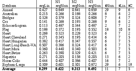
In order to determine whether each normalization scheme N1, N2 and N3 gave unfair weight to either nominal or linear attributes, experiments were run on 15 databases from the machine learning database repository at the University of California, Irvine (Merz & Murphy, 1996). All of the datasets for this experiment have at least some nominal and some linear attributes, and thus require a heterogeneous distance function.
In each experiment, five-fold cross validation was used. For each of the five trials, the distance between each instance in the test set and each instance in the training set was computed. When computing the distance for each attribute, the normalized_diff function was used for linear attributes, and the normalized_vdm function N1, N2, or N3 was used (in each of the three respective experiments) for nominal attributes.
The average distance (i.e., sum of all distances divided by number of comparisons) was computed for each attribute. The average of all the linear attributes for each database was computed and these averages are listed under the heading "avgLin" in Table 1. The averages of all the nominal attributes for each of the three normalization schemes are listed under the headings "avgNom" in Table 1 as well. The average distance for linear variables is exactly the same regardless of whether N1, N2 or N3 is used, so this average is given only once. Table 1 also lists the number of nominal ("#Nom.") and number of linear ("#Lin.") attributes in each database, along with the number of output classes ("#C").
 |
Table 1. Average attribute distance for linear and nominal attributes.
As can be seen from the overall averages in the first four columns of the last row of Table 1, N2 is closer than N1 or N3. However, it is important to understand the reasons behind this difference in order to know if the normalization scheme N2 will be more robust in general.
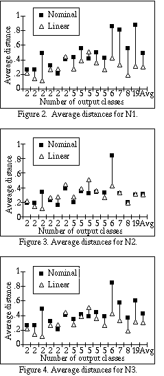
 Figures 2-4 graphically display the averages shown in Table 1 under the
headings N1, N2 and N3, respectively, ordered from left to right by the number
of output classes. We hypothesized that as the number of output classes grows,
the normalization would get worse for N3 if it was indeed not appropriate to
add the scaling factor C to the sum. The length of each line indicates
how much difference there is between the average distance for nominal
attributes and linear attributes. An ideal normalization scheme would have a
difference of zero, and longer lines indicate worse normalization.
As the number of output classes grows, the difference for N3 between the linear distances and the nominal distances grows wider in most cases. N2, on the other hand, seems to remain quite close independent of the number of output classes. Interestingly, N1 does almost as poorly as N3, even though it does not use the scaling factor C. Apparently the squaring factor provides for a more well-rounded distance metric on nominal attributes similar to that provided by using Euclidean distance instead of Manhattan distance on linear attributes.
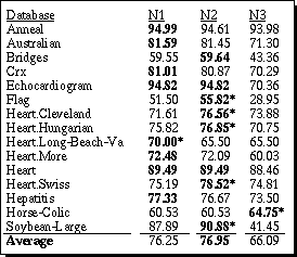
The underlying hypothesis behind performing normalization is that proper normalization will typically improve generalization accuracy. A nearest neighbor classifier (with k=1) was implemented using HVDM as the distance metric. The system was tested on the heterogeneous datasets appearing in Table 1 using the three different normalization schemes discussed above, using ten-fold cross-validation (Schaffer, 1993), and the results are summarized in Table 2. All the normalization schemes used the same training sets and test sets for each trial. Bold entries indicate which scheme had the highest accuracy. An asterisk indicates that the difference was greater that 1% over the next highest scheme.
As can be seen from the table, the normalization scheme N2 had the highest accuracy, and N1 was substantially lower than the other two. N2 and N3 each had the highest accuracy for 8 domains. More significantly, N2 was over 1% higher 5 times compared to N1 being over 1% higher on just one dataset. N3 was higher than the other two on just one dataset, and had a lower average accuracy than N2.

Table 2. Generalization accuracy using N1, N2 and N3.
These results support the hypothesis that the normalization scheme N2 achieves higher generalization accuracy than N1 or N3 (on these datasets) due to its more robust normalization though accuracy for N3 is almost as good as N2.
Note that proper normalization will not always necessarily improve generalization accuracy. If one attribute is more important than the others in classification, then giving it a higher weight may improve classification. Therefore, if a more important attribute is given a higher weight accidentally by poor normalization, it may actually improve generalization accuracy. However, this is a random improvement that is not typically the case. Proper normalization should improve generalization in more cases than not when used in typical applications.
As a consequence of the above results, N2 is used as the normalization scheme for HVDM, and the function normalized_vdm is defined as in (15).
A nearest neighbor classifier (with k=1) using the three distance functions listed in Table 3 was tested on 48 datasets from the UCI machine learning database repository. Of these 48 datasets, the results obtained on the 35 datasets that have at least some nominal attributes are shown in Table 3.
The results are approximately equivalent on datasets with only linear attributes, so the results on the remaining datasets are not shown here, but can be found in Section 6. 10-fold cross-validation was again used, and all three distance metrics used the same training sets and test sets for each trial.
The results of these experiments are shown in Table 3. The first column lists the name of the database (".test" means the database was originally meant to be used as a test set, but was instead used in its entirety as a separate database). The second column shows the results obtained when using the Euclidean distance function normalized by standard deviation on all attributes, including nominal attributes. The next column shows the generalization accuracy obtained by using the HOEM metric, which uses range-normalized Euclidean distance for linear attributes and the overlap metric for nominal attributes. The final column shows the accuracy obtained by using the HVDM distance function which uses the standard-deviation-normalized Euclidean distance (i.e., normalized_diff as defined in Equation 13) on linear attributes and the normalized_vdm function N2 on nominal attributes.
The highest accuracy obtained for each database is shown in bold. Entries in the Euclid. and HOEM columns that are significantly higher than HVDM (at a 90% or higher confidence level, using a two-tailed paired t test) are marked with an asterisk (*). Entries that are significantly lower than HVDM are marked with a "less-than" sign (<).
 |
Table 3. Generalization accuracy of the
Euclidean, HOEM, and HVDM distance functions.
As can be seen from Table 3, the HVDM distance function's overall average accuracy was higher than that of the other two metrics by over 3%. HVDM achieved as high or higher generalization accuracy than the other two distance functions in 21 of the 35 datasets. The Euclidean distance function was highest in 18 datasets, and HOEM was highest in only 12 datasets.
HVDM was significantly higher than the Euclidean distance function on 10 datasets, and significantly lower on only 3. Similarly, HVDM was higher than HOEM on 6 datasets, and significantly lower on only 4.
These results support the hypothesis that HVDM handles nominal attributes more appropriately than Euclidean distance or the heterogeneous Euclidean-overlap metric, and thus tends to achieve higher generalization accuracy on typical applications.
Return to Contents
Send comments to randy@axon.cs.byu.edu